More Examples

Tapped Delay Neural Network - Sunspot example

A time serie is a sequence of vectors, that depend on time .

The time series could also consist of a sequence of scalars .

This example based upon an exercise 4 from a IMM, DTU course on signal processing [imm02457]. The examples is located in PyPR’s examples folder, in a subfolder called sunspots.

#!/bin/python

# This code is based upon the exerice 4 from the IMM DTU course 02457
# written by Lars Kai Hansen & Karam Sidaros

from numpy import *
import pypr.preprocessing as preproc
import pypr.ann as ann
import pypr.optimization as opt
from pypr.helpers.modelwithdata import *
from pypr.stattest import *

# Load data
rg = genfromtxt('sp.dat')
year = rg[:,0].astype(int)
sp = rg[:,1]

d = 3 # Number of inputs
train_until_year = 1920 # including
last_train = nonzero(year==train_until_year)[0][0]-d

# Create lag space matrix 
N = len(year)-d
T = np.c_[sp[d:]]
X = ones((N,d))
for a in range(0, N):
  X[a,:] = sp[a:a+d]

# Training and test sets
Xtrain=X[0:last_train+1,:]
Ttrain=T[0:last_train+1,:]
Xtest=X[last_train+1:,:]
Ttest=T[last_train+1:,:]

# Normalize:
normX = preproc.Normalizer(Xtrain)
normT = preproc.Normalizer(Ttrain)
Xn = normX.transform(X)
Tn = normT.transform(T)
Xtrain_n = normX.transform(X)
Ttrain_n = normT.transform(T)

# Setup model:
#nn = ann.WeightDecayANN([d, 4, 1])
nn = ann.WeightDecayANN([d, 20, 1])
nn.v = 0.0 # Weight decay, just a guess, should actually be found
dm = ModelWithData(nn, Xtrain_n, Ttrain_n)

# Train model:
err = opt.minimize(dm.get_parameters(), dm.err_func, dm.err_func_d, 500)

# Predict
Y = normT.invtransform(nn.forward(Xn))
SE = (Y-T)**2.0

# Plot data
figure()
subplot(211)
plot(year, rg[:,1], 'b', label='Target')
title('Yearly mean of group sunspot numbers')
xlabel('Year')
ylabel('Number')
plot(year[d:], Y, 'r', label='Output')
legend()
title('Sunspot predcition using a NN with %d inputs'%d)
axvline(train_until_year)
subplot(212)
plot(year[d:], SE)
xlabel('Year')
ylabel('$(y(x^n)-t^n)^2$')
title('Mean square error = %.2f'%np.mean(err))

# Plot sample autocorrelation of the residual of the fitted model
figure()
lags = range(0,21)
stem(lags, sac(Y-T, lags))
title('Sample Autocorrelation of residuals')
xlabel('Lag')
ylabel('Sample Autocorrelation')

The example should generate a plot similar similar to this:

And a plot with the sample autocorrelation of the fitted models residuals.

[imm02457]

02457 Nonlinear Signal Processing, http://cogsys.imm.dtu.dk/teaching/04364/04364prac.html

Gaussian Mixture Model Regression (GMR) - Sunspot example

#!/bin/python

# This code is based upon the exerice 4 from the IMM DTU course 02457
# written by Lars Kai Hansen & Karam Sidaros

from numpy import *
import numpy as np
from scipy import *
import pypr.clustering.gmm as gmm
import pypr.preprocessing.lag_matrix as lm
from pypr.stattest import *

# Load data
rg = genfromtxt('sp.dat')
year = rg[:,0].astype(int)
sp = rg[:,1]

d = 11 # Number of inputs
train_until_year = 1920 # including
last_train = nonzero(year==train_until_year)[0][0]-d

X = lm.create_lag_matrix(np.c_[sp], d)

# Training and test sets
Xtrain=X[0:last_train+1,:]
Xtest=X[last_train+1:,:]

cluster_init_kw = {'cluster_init':'kmeans', 'max_init_iter':5, \
    'cov_init':'var', 'verbose':True}
cen_lst, cov_lst, p_k, logL = gmm.em_gm(Xtrain, K = 5, max_iter = 200, \
    delta_stop=1e-5, init_kw=cluster_init_kw, verbose=True)

# Predict
T = np.c_[X[:,-1]]
Y = np.zeros(T.shape)
for i in range(len(Y)):
    cond_input = np.concatenate((X[i,:-1], np.nan*np.ones(1)))
    cen_cond, cov_cond, mc_cond = gmm.cond_dist(np.array(cond_input),\
        cen_lst, cov_lst, p_k)
    for j in range(len(cen_cond)):
        Y[i] = Y[i] + (cen_cond[j]*mc_cond[j])

SE = (Y-T)**2.0

# Plot data
figure()
subplot(211)
plot(year, rg[:,1], 'b', label='Target')
title('Yearly mean of group sunspot numbers')
xlabel('Year')
ylabel('Number')
plot(year[d:], Y, 'r', label='Output')
legend()
title('Sunspot predcition using a NN with %d inputs'%d)
axvline(train_until_year)
subplot(212)
plot(year[d:], SE)
xlabel('Year')
ylabel('$(y(x^n)-t^n)^2$')
title('Mean square error = %.2f'%np.mean(SE))

# Plot sample autocorrelation of the residual of the fitted model
figure()
lags = range(0,21)
stem(lags, sac(Y-T, lags))
title('Sample Autocorrelation of residuals')
xlabel('Lag')
ylabel('Sample Autocorrelation')

# Predict the future (pass outputs from the ANN to the inputs)
curr_input = Xtest[0, :-1]
res = [Ttest[0,0]]
for i in range(1, len(Ttest)):
    print curr_input
    cond_input = np.concatenate((curr_input, np.nan*np.ones(1)))
    cen_cond, cov_cond, mc_cond = gmm.cond_dist(np.array(cond_input),\
        cen_lst, cov_lst, p_k)
    pred = 0
    for j in range(len(cen_cond)):
        pred = pred + (cen_cond[j]*mc_cond[j])
    curr_input = np.concatenate((curr_input[1:], pred.flatten()))
    res.append(pred)
figure(figsize=(8,3))
plot(year[-len(res):], res, 'r--', label='Predicted')
plot(year, rg[:,1], 'b', label='Target')
axvline(year[-len(res)])
xlabel('Year')
ylabel('Number')

Finding the Number of Clusters to use in a Gaussian Mixture Model

# Drawing samples from a Gaussian Mixture Model
from numpy import *
from matplotlib.pylab import *
import pypr.clustering.gmm as gmm
import pypr.stattest as stattest

seed(10)
mc = [0.4, 0.4, 0.2] # Mixing coefficients
centroids = [ array([0,0]), array([3,3]), array([0,4]) ]
ccov = [ array([[1,0.4],[0.4,1]]), diag((1,2)), diag((0.4,0.1)) ]
    # Covariance matrices

T = gmm.sample_gaussian_mixture(centroids, ccov, mc, samples=500)
V = gmm.sample_gaussian_mixture(centroids, ccov, mc, samples=500)
plot(T[:,0], T[:,1], '.')

# Expectation-Maximization of Mixture of Gaussians
Krange = range(1, 20 + 1);
runs = 1
meanLogL_train = np.zeros((len(Krange), runs))
meanLogL_valid = np.zeros((len(Krange), runs))
for K in Krange:
    print "Clustering for K = ", K; sys.stdout.flush()
    for r in range(runs):
        cen_lst, cov_lst, p_k, logL = gmm.em_gm(T, K = K, iter = 100)
        meanLogL_train[K-1, r] = logL
        meanLogL_valid[K-1, r] = gmm.gm_log_likelihood(V, cen_lst, cov_lst, p_k)

fig1 = figure()
subplot(1, 2, 1)
for r in range(runs):
    plot(Krange, meanLogL_train[:, r], 'g:', label='Training')
    plot(Krange, meanLogL_valid[:, r], 'b-', label='Validation')
legend(loc='lower right')
xlabel('Number of clusters')
ylabel('log likelihood')

bic = np.zeros(len(Krange))
# We should train with ALL data here
X = np.concatenate((T,V), axis = 0)
meanLogL_full = np.zeros(len(Krange))
for i, K in enumerate(Krange):
    print "Clustering for K = ", K; sys.stdout.flush()
    for r in range(runs):
        cen_lst, cov_lst, p_k, logL = gmm.em_gm(X, K = K, iter = 100)
        meanLogL_full[i] += logL
meanLogL_full /= runs
for i, K in enumerate(Krange):
    D = 2
    M = (K-1) + K*(D+0.5*D*(D+1))
    N = X.shape[0]
    bic[i] = stattest.bic(meanLogL_full[i], M, N)
subplot(1, 2, 2)
plot(Krange, bic)
xlabel('Number of clusters')
ylabel('BIC score')

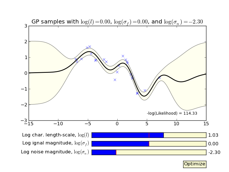
Simple GP demo

In the examples folder you can find a program called ‘gp_hyperparameters_demo.py’ where the effects of the GP’s hyperparameters are illustrated.

Multiclass classification using ANN

# Example using the Iris dataset for multiclass classification
# Dataset obtained from: http://archive.ics.uci.edu/ml/datasets/Iris

# From UCI Machine learning repository:
# Attribute Information:
#
# 1. sepal length in cm 
# 2. sepal width in cm 
# 3. petal length in cm 
# 4. petal width in cm 
# 5. class: 
# -- Iris Setosa 
# -- Iris Versicolour 
# -- Iris Virginica

import numpy as np
import pypr.preprocessing as preproc
import pypr.ann as ann
import pypr.ann.activation_functions as af
import pypr.ann.error_functions as ef
import pypr.optimization as opt
import pypr.helpers as help

plant_names = ['Iris-setosa', 'Iris-versicolor', 'Iris-virginica']
converters = {4: plant_names.index}
data = np.loadtxt('iris/iris.data', delimiter=',', converters=converters)
C_no = np.c_[data[:,4]]

inputCol = [0, 1, 2, 3]
X = data[:, inputCol]
T = np.concatenate((Cno==0, Cno==1, Cno==2), axis=1) * 1.0

# Normalize:
normX = preproc.Normalizer(X)
Xn = normX.transform(X)

# Setup model:
hidden_neurons = 8 # This should be enough to overfit the problem
nn = ann.WeightDecayANN([len(inputCol), hidden_neurons, T.shape[1]],
                        [af.tanh, af.softmax], errorfunc=ef.entropic)
nn.v = 0.0 # Weight decay, just a guess, should actually be found
dm = help.ModelWithData(nn, Xn, T)

# Train model:
err = opt.minimize(dm.get_parameters(), dm.err_func, dm.err_func_d, 300)

Y = nn.forward(Xn)
predicted_C_no = np.argmax(Y, axis=1) # Assign number to each group again
success = np.c_[predicted_C_no] == C_no
total_correct = np.sum(success)

print "Correct predictions =", total_correct
print "Incorrect predictions =", len(success) - total_correct

When runned the program will generate an output similar to this:

>>> execfile('iris.py')
Correct predictions = 150
Incorrect predictions = 0